At HSS we are quite comfortable with our status as an emerging seismic processing service provider. Part of the territory therefore is that most of our work to date has taken place in the time domain whilst leaving the depth processing work to our more established competitors. This is something that is about to change!

Several enquires at the recent AEGC 2019 made us realise that there was an opportunity to provide some depth migration services if we add the requisite algorithms to our toolbox. Depth imaging has always been on our radar so there was a tentative plan already sketched out and I already had a good idea about what software “parts” would be required. The only thing that has been missing to this point has been sufficient priority to warrant investing the time to make it happen. Having potential projects in the pipeline is all the impetus we needed to fast track this development.

There are a lot of algorithms that can be implemented in pursuit of excellence in depth imaging but the most fundamental being a robust and accurate Kirchhoff style migration algorithm. To this end it is important to be able to create accurate synthetic datasets for the purpose of testing the migration – if it won’t work on synthetics it won’t work on real data! So the first two milestone stages on our path to being a depth imaging service provider as I see it are 1) forward modelling some synthetic seismic data for a given model and 2) being able to accurately image this synthetic data back into the depth domain.

Forward Modelling

Everyone’s got a hobby. I have always really enjoyed creating synthetic seismic data. The upshot of spending many hours writing algorithms for creating synthetic seismograms is that I already had a few options when it came to this step. Looking at the problem we are trying solve by depth migration (and therefore the problem we are trying to produce by forward modelling) it made sense to dig out my kinematic ray tracing code. For a given model it will calculate arrival times for ray paths from any source to receiver through a given model. The model (clearly) needs to be supplied as well as the name of horizons which one would like rays to reflect off (as opposed to transmit through).

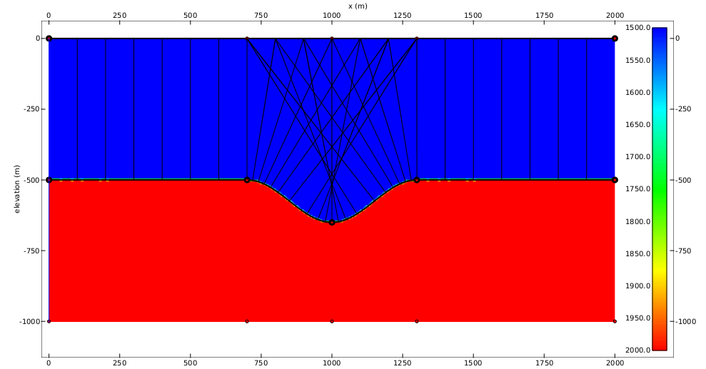
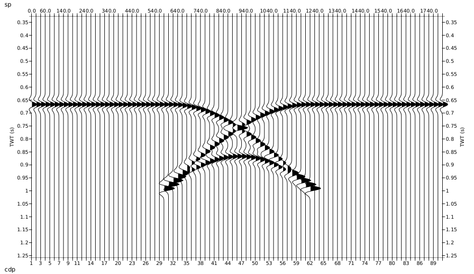
Even though I thought this code was almost good to go there were the inevitable complications that led to a bit of debugging. After a few hours of work I managed to produce the classic bow-tie normal incidence section that one expects from a syncline. And I was happy.

Migration

Now that we can produce the problem it’s time to work on solving it. This side of things is where I have spent far less time playing around. Our current Kirchhoff migration algorithm works in the time domain only. The exciting thing about working in the depth domain is that a correctly working depth migration algorithm will image the model in the same domain that it was created so checking the accuracy should be absolutely straight forward.

At the heart of a Kirchhoff depth migration algorithm you will always find a method of calculating the travel time from a given source to a given receiver for all possible reflection points in the model. A problem becomes apparent. There are many possible travel paths from a given source to receiver. Which one should we choose? The first? The most energetic?

For a first implementation I have chosen to go simply for the first arrival. The reason for this is that whilst playing with synthetics (yay!) and tomography a couple of years ago I had written an Eikonal equation solver and solving the Eikonal equation essentially calculates the first arrival times at any given point. So once again I could simply plug in some already written code. Fortunately this part of the code worked without any additional attention.

With the ability to calculate travel times throughout a model the Kirchhoff PSDM algorithm then looks a little something like this:

For each input trace:
    t_s: travel time from source to every point in the model
    t_r: travel time from receiver to every point in the model
    t_total=t_s+t_r: reflection time to every point in the model
    For each output trace location:
        For each depth:
            Get the travel time from t_total
            Use this time to interpolate a value from input trace
            Sum this interpolated value into the migration image

And that’s pretty much it. Now to find a home for this new code. I have never seen time and depth migration algorithms implemented within the same module (let me know if you have) and that’s always made a lot of sense to me. However, when I came to the point of implementing this algorithm I saw how much overlap there was going to be with my existing time migration code. And because hate code duplication I simply added a “domain” parameter to the existing migration module and stuck the new code in there. And thus with comfortably fewer than 30 new lines of code we now have depth migration!

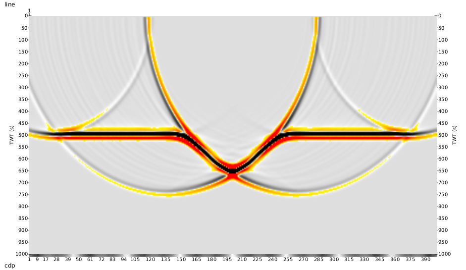
I ran the zero offset data from above through the depth migration and achieved the result below. Pleasingly the single reflector is at the correct depth and the syncline is the correct shape. Clearly there are some cancellation issues but I’m not too concerned at this stage. All this means is that the migration is not the perfect adjoint operation to the modelling. As more realism goes into both the modelling and the migration this result will improve.

On the agenda

As happy as I am with the progress to this point there’s still a lot of work to do:

• Add more sophistication to the modelling: geometric spreading, caustic phase changes etc.
• Progress to 3D modelling and migration
• Write a residual moveout picker add-on to our velocity picker app
• Write a tomography module that converts these residual moveout picks to a model update
• Add a whole raft of other features into our depth model building app to allow for the quasi interpretative work flow required during a depth migration project (e.g. horizon velocity analysis, flood fill for intrusive bodies etc).

So there’s plenty to keep me going. Stay tuned!